

Download the applet
Click HERE to download the applet of 3RRR robot simulator.
You can also run the applet below. Users of Mac Lion 10.7.4 OS might encounter problems when trying to run it directly in the browser and may need to download the jar file.
Instructions of use
The features of this simulator are these: forward and inverse kinematics, singularity analysis and workspace visualization. There is a keypad column on the left side of the window where the user can choose what kind of analysis is to be performed, and where the sizes of the links of the robot can be modified. A graphical window on the right-hand side of the applet shows a schematic representation of this parallel mechanism (see figure 1). The position of the fixed supports of the robot can be changed dragging them with the mouse in this graphical window.
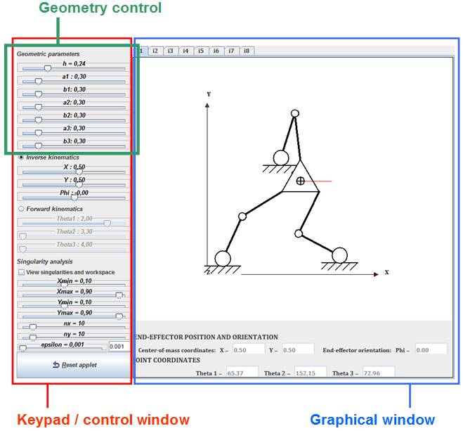
Figure 1. Main parts of the applet.
The geometric parameters that define the robot and whose value can be modified in the control window correspond to the dimensions specified in figure 2:
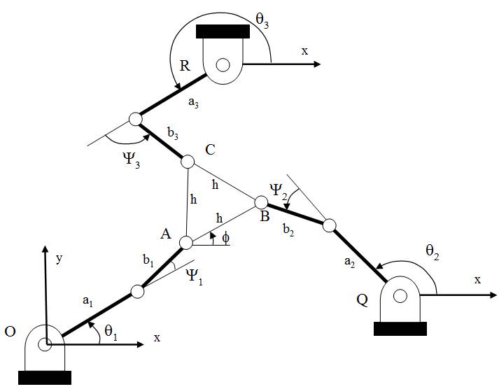
Figure 2. Explanation of the main geometric parameters that can be modified in the applet.
When inverse kinematics analysis is chosen, the user establishes the cartesian (x, y) coordinates of the centre of mass of the end-effector and its orientation (angle Φ depicted in figure 2) and the application computes the values of the joint angles, giving an amount of 8 different inverse kinematic solutions. These different solutions can be selected from the tabs in the top part of the graphics window. The input variables for the inverse kinematics (position of the end-effector and its orientation) can be changed either by moving the slide bars in the keypad or by clicking on the moving platform. By clicking and dragging the centre of mass of the platform the user can modify the position of the end-effector without any change in its orientation. To change the orientation of the moving platform, there is a thin red line attached to that platform that the user can pick and rotate about the platform centre of mass. At any time, at the bottom part of the graphics window the cartesian coordinates of the platform and the joint angles obtained from the inverse kinematic problem solution are displayed for the current inverse solution (see figure 3).
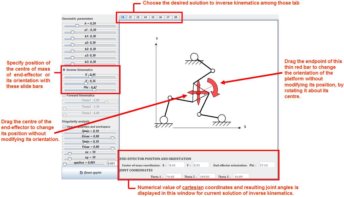
Figure 3. View of the applet when performing an inverse kinematics analysis.
While the inverse
kinematics menu is active, a singularity and workspace analysis can be done. At
the bottom part of the keypad column of the application are some sliding bars
to handle workspace and singularity computation and visualization. First the
user should activate the feature by marking the associated tick, which enables
the visualization and calculation of the singularities. When doing so, in the
graphics window where the robot is displayed will appear some lines and a box.
This box encloses the area where an algorithm will perform a sweep over the
space of inverse kinematics solutions to search for the singular
configurations, and its limits can be changed either by moving the vertices of
the box by dragging them with the mouse or by the use of sliding bars situated
at the keypad menu (parameters Xmin,
Xmax, Ymin and Ymax). The number
of points in which the enclosed space of the box will be divided in both x and
y axes in the discretization is specified by the sliding bars with the labels 'nx' and 'ny'. Finally, there is a slide bar labelled 'epsilon' that corresponds with the threshold value such that any
point that generates a Jacobian matrix whose determinant is under that
threshold will be classified as a singular configuration. In order to visualize
properly singular points in the x-y space of the robot, this threshold should
be set to 0.0001-
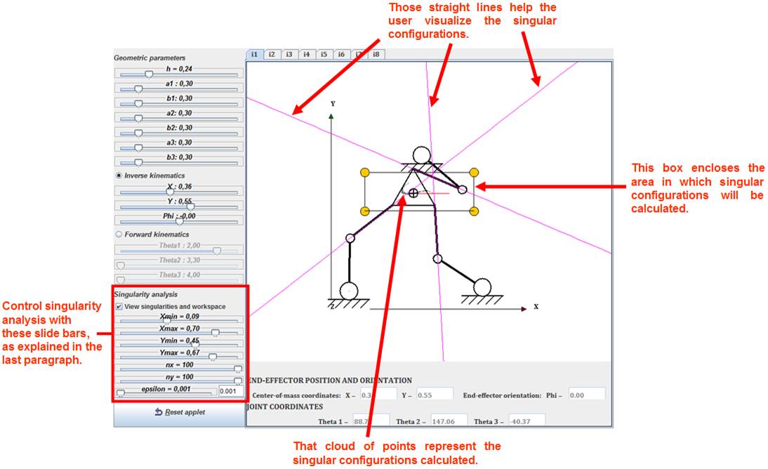
Figure 4. Example of a singular configuration. The algorithm sweeps the area enclosed by the box and searches for singularities inside that box. In the example shown, the centre of the end-effector has been positioned on a singular point. Those singularities correspond to configurations in which the three pink straight lines intersect in one point. In that configuration, the end-effector gains instantaneously one or more degrees of freedom. The pink lines are the extension of links b1, b2 and b3 as defined in figure 2.
As for the function of the thin pink lines that also appear when singularities are shown (see figure 4), their objective is to aid the user visualize the singularities. Inverse kinematic singularities correspond to the points at the boundary of the workspace, while forward kinematic singularities are found inside that workspace. For the 3RRR robot studied, direct singular configurations are attained when either the three lines along the links of lenght b1, b2 and b3 (the pink lines shown in the simulator) intersect at the same point or when those lines are parallel. When displaying only forward singularities (i.e. taking a sufficiently small threshold such as epsilon = 0.001) the user can check this by locating the centre-of-mass of the end-effector on the singular points calculated by the simulation and check if those conditions are actually met in the singularities, looking at the relative position of the straight pink lines.
Singularity and workspace analysis is not available when the forward kinematics feature is active. If the user selects the forward kinematics analysis, then position and orientation of the moving platform is computed and displayed in the graphics window for the chosen joint angles. The input angles can be introduced by sliding bars or manually rotating the input links dragging their passive joint with the mouse (see figure 5).
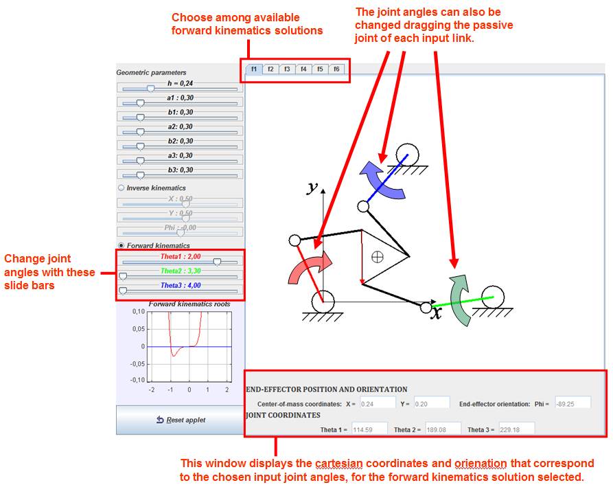
Figure 5. Aspect of the applet when performing forward kinematics analyses.
An important difference between the direct kinematic problem of 3RRR robot and the same problem for the Delta and 5R robots is that in general there is not an analytical solution for 3RRR forward kinematics. The solution to the direct kinematics of 3RRR robot requires finding the roots of an eigth-degree polynomial on tan(Φ/2), i.e. a polynomial of the form:

Where Φ is the orientation of the platform as seen in figure 2. After Φ is known, the x and y coordinates of the center-of-mass of the moving platform are computed easily. From the degree of the previous polynomial we may expect 8 different solutions from the forward kinematic problem. However, it can be proved by geometric arguments that the preceding equation can have 6 real solutions at most. Since we can expect to find at most 6 real angles the user can choose among 6 tabs which solution should be displayed. Nevertheless, in general we will not have all the 6 solutions available because the selected robot dimensions and input angles may lead only to a pair of real solutions, being the rest complex solutions. In that case, a message is displayed in the window where the solution is shown to warn the user that the actual solution displayed is not correct since the found angle is not real but complex (see figure 6). To help the user study forward kinematics problem in the simulator, the polynomial in the previous equation is continuously plotted to show how many times does the polynomial cross the y=0 line and thus visualize how many real roots are we obtaining. Moreover, the polynomial plotted evolves and changes automatically as geometric parameters of the robot or input joint angles change, so the user can see how those changes affect the forward kinematic problem. The polynomial roots are found using a numerical procedure.
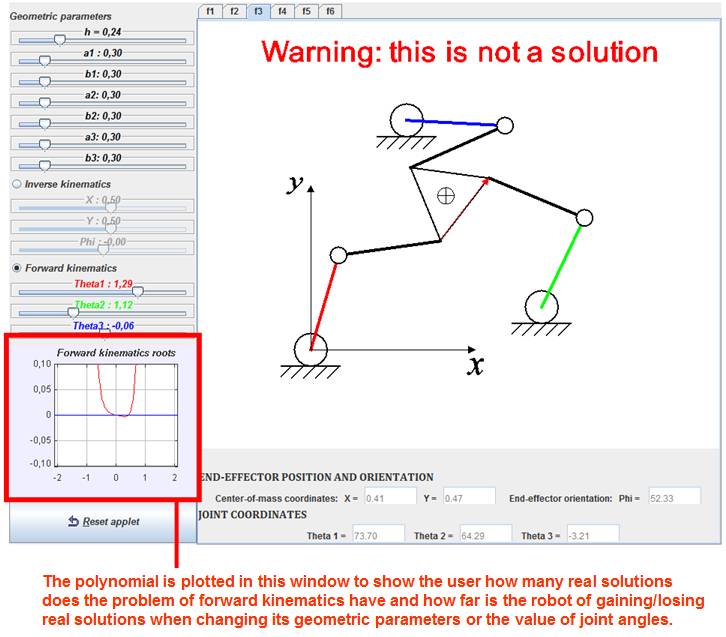
Figure 6. The polynomial that yields the forward kinematic solutions is plotted in the shown window. Moreover, a warning message is displayed when a selected forward kinematics solution is false because it correspond to complex values of the angle Φ. In the example shown, only two solutions are real (solutions in tabs 'f1' and 'f2'). The polynomial only crosses the y=0 line twice.