

The kinematics of 5R robot can be simulated with the applet shown below. Java Applet Plug-in of the bowser will have to be active in order to play the applet.
You can also DOWNLOAD this applet.
1. Instructions of use
This applet is divided into two areas: a 2D-graphics window on the left-hand side of the application and a control window on its right-hand side. The graphics window is again divided in two parts, the one on the left-hand side shows a scheme of the 5R parallel robot in cartesian space while the other displays the current value of the actuated joints of the robot (values of θ1 and θ2) as a point in the joint space (the range of the angles shown in this space is [-π, π]). The user can change the size of each window dragging the vertical bars that separate them. Figure 1 depicts this configuration.
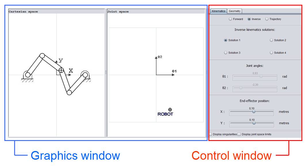
Figure 1. Overview of the applet.
The user can interact with the applet by clicking either in the control window or in the graphics window. When using the control window the user can choose between performing some kinematic simulations (forward and inverse kinematics or trajectory analysis) and changing the lengths of the bars that comprise the mechanism. This choice can be made by means of the tabs located at the top part of the control window, as figure 2 shows. As can be seen in that picture, in the ‘Geometry’ tab the lengths of the links can be changed by sliding bars. There is also a schematic picture of the robot which acts as a key to help the user. Besides being able to change the length of the links, the position of the supports of the robot can also be changed by dragging them with the mouse in the graphics window.
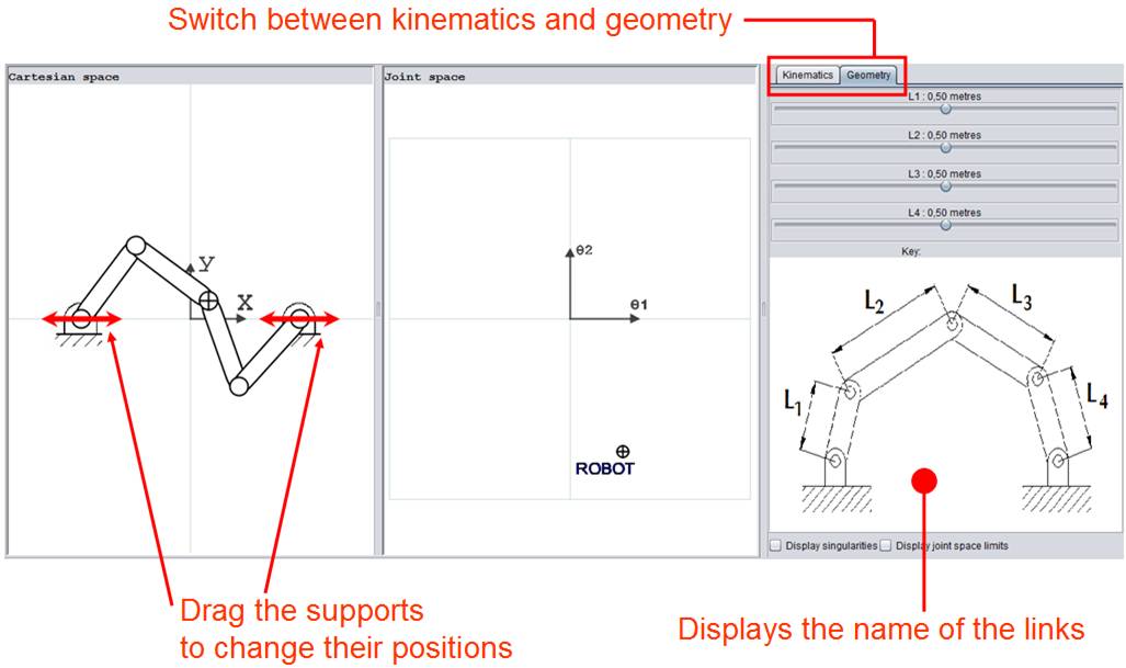
Figure 2. Changing the geometric parameters of the robot (lengths of the links and position of the supports).
If a kinematic analysis is to be performed (‘Kinematics’ tab is active), the user must choose among simulating the forward kinematics, the inverse kinematics and a trajectory analysis of the robot. The features of each simulation will be described in the following sections.
2. Inverse kinematics analysis
Inverse kinematics is the problem of finding the values of the actuated joints of the robot that yield a specified end-effector position. For this 2-DOF parallel robot, when we impose the position of the end-effector (x and y coordinates of the end-effector of the mechanism) there are 4 different combinations of joint angles that locate the end-effector in the desired position. The user can choose which one of the four solutions to the inverse kinematics problem is to be simulated by selecting a switch. The resulting values of joint angles are displayed in the ‘Joint angles’ window of the control window (see figure 3). The position of the end-effector is modified by dragging it in the graphics window (which allows the user to modify the x coordinate of the end-effector and its y coordinate simultaneously) or using the sliding bars in the control window(only one coordinate will be modified at a time, either x or y). The specified position has metres units.
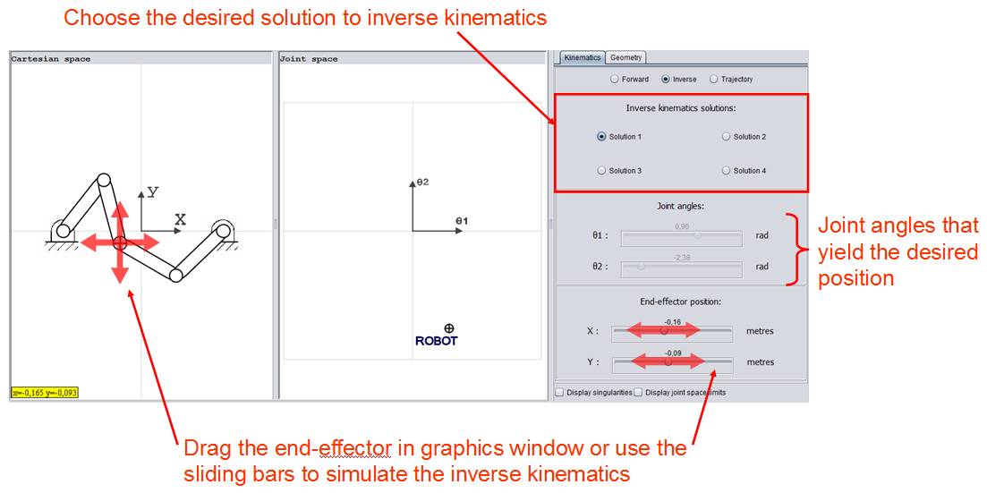
Figure 3. Simulation of the inverse kinematics of the 5R robot.
3. Forward kinematics analysis
When we specify the values of the actuated joints of the robot instead of the position of its end-effector, we have to solve the forward kinematics problem. Solving this problem allows us to know the position of the end-effector (its x and y coordinates) in terms of the joint angles θ1 and θ2. There are two different positions of the end-effector of this robot when we specify the values of the joint angles and thus we say that there are two solutions for the forward kinematics of the 5R robot. Similarly to the simulator of inverse kinematics, the desired solution to forward kinematics can be switched in the ‘Forward kinematics solutions’ window of the control window (see figure 4). When one of the two available solutions is chosen, the resulting value of the x and y coordinates of the end-effector will be displayed in the ‘End-effector position’ of the control window (since the coordinates x and y are now the output of the simulation, they cannot be modified in this case neither by dragging the end-effector in the graphics window or by the sliding bars of this sub-window).
The value of the actuated joint angles (input to the simulation) can be modified in two ways: dragging the point labeled ‘ROBOT’ in the ‘Joint space’ window of the graphics window (both angles – θ1 and θ2 – can be modified at a time) or moving the sliding bars in the sub-window ‘Joint angles’ of the control window. In both cases, the units of the input are radians.
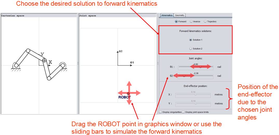
Figure 4. Simulation of forward kinematics of the 5R robot.
4. Trajectory analysis
In addition to the simulation of the forward and inverse kinematics, this applet also supports the simulation of trajectories in the workspace of the robot. When choosing this analysis in the simulator, two points appear in the ‘Cartesian space’ graphical window. Those points are labeled ‘START’ and ‘GOAL’ and are the initial and final points of the desired trajectory, respectively. When the user defines the position of the extreme points of the trajectory in the cartesian space (either by dragging those points in the x-y plane or by introducing manually the coordinates of the points in the control menu), the robot will perform a trajectory that connects both points after pressing the ‘Launch trajectory’ button. Before launching the trajectory, the solution to the forward kinematics that will be used to simulate the trajectory must be selected.
It should be mentioned at this point that the simulator can also calculate the singularities of the robot and display them in the cartesian and joint spaces of the graphical window. The singularities of a parallel robot are those configurations for which any of the Jacobian matrices that relate the joint and cartesian velocities (or both matrices) become singular. They can be classified in singularities of forward kinematics and singularities of inverse kinematics. On the one hand, forward kinematics singularities occur inside the workspace of the robot and are those points for which the forward kinematics problem degenerates and both solutions are the same. On the other hand, inverse kinematics singularities lie in the boundary of the workspace of the robot and in those configurations some of the inverse kinematics solutions coincide. Activating the tick ‘Display singularities’ at the bottom of the control window simulator will display the inverse kinematics singularities (i.e. the limits of the workspace of the robot) in the cartesian space. If the user is simulating inverse kinematics, the singularities of forward kinematics will also be shown in the cartesian space (singularities inside the workspace) – it will show only those forward kinematics singularities that are approached with current inverse kinematics solution (the user can then check that in the resulting points both forward kinematics coincide, which means that the links L2 and L3 are parallel).
Activating the tick ‘Display joint space limits’ at the bottom of control window will display in joint space the forward kinematics singularities. While the inverse kinematics singularities lie in the boundary of the workspace and the forward kinematics singularities lie within that workspace in cartesian space, in joint space those roles are swapped: forward kinematics singularities define the limits of the ‘joint workspace’ (which could be defined as the set of values of the actuated joints for which there exists at least one solution for forward kinematics) and the singularities of inverse kinematics remain inside those boundaries (the applet does not show them for current version, however). The importance of this ‘joint workspace’ is that it helps in the simulation of forward kinematics, since the user can know at every moment which pairs of input angles guarantee a solution of forward kinematics problem. But its utility goes beyond this – in this case, the path-planning algorithm that the simulator uses searches for a trajectory in the joint workspace, as we will see later. Figure 5 shows the way in which the applet displays the singularities in both spaces – cartesian space and joint space.
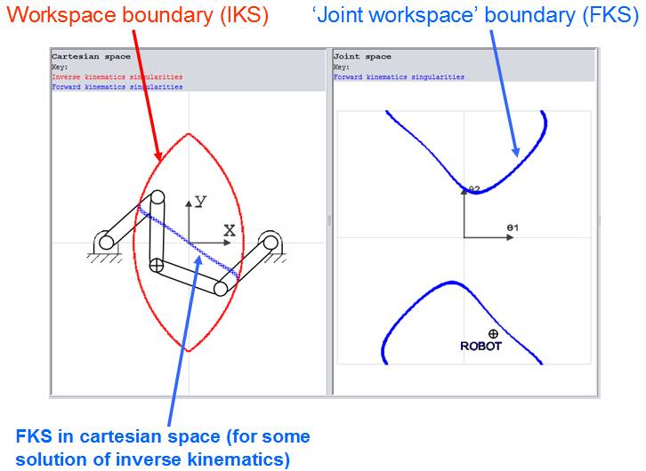
Figure 5. Inverse kinematics singularities (red) and forward kinematics singularities (blue) shown in cartesian and joint spaces. Note: IKS = inverse kinematics singularities. FKS = forward kinematics singularities.
For the trajectory analysis, it is important to note that the robot won’t be able to attain every point in the cartesian space. The robot will only be able to approach those points that lie within its workspace, which in general is the intersection of two annulus, as shown in the left-hand side of figure 5. Moreover, not every point of the workspace can be attained with a single solution of the forward kinematics problem. This means that the robot won’t be able to describe some trajectories even when its endpoints lie inside its workspace, for it would need to change from one forward kinematic solution to the other in the middle of the trajectory. Figure 6 shows an example of this situation.
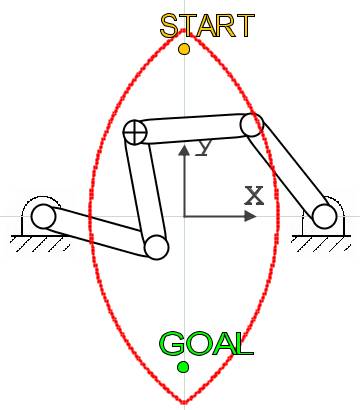
Figure 6. Example of an impossible trajectory: the START and GOAL points cannot be reached with the same solution of forward kinematics. The robot would need to change its assembly mode in order to perform the desired trajectory.
Since not every trajectory is possible, when the user defines the start and goal points the applet checks if both points are attainable with the selected solution of forward kinematics (which also includes checking if the mentioned points lie within the workspace of the robot). If the trajectory can be performed, then the ‘Launch trajectory’ is available and pressing it will start the path-planning algorithm and, eventually, the simulation of the resulting trajectory. In case any of the points is not reachable, the applet will not allow the user to launch the trajectory until valid extreme points are chosen (the applet tells the user at every time the state of the start and goal points – valid>, unreachable with current assembly or out of the workspace). The possibility of displaying the workspace acquires a big importance here, for the user can visualize better those points which are attainable. Moreover, when the length of any of the links is modified or the position of any of the supports is changed the workspace shape will change, providing an interesting tool for the process of design of parallel structures.
When both start and goal points are reachable with the selected solution of forward kinematics, the trajectory will start after pressing the button ‘Launch trajectory’, at the bottom of the control window. After this button has been pressed, the user won’t be able to change anything in the applet until the simulation of the trajectory has finished (changes in type of analysis, endpoints, position of supports or length of the links will be forbidden). In the path-planning algorithm, the applet will first find a feasible path that connects the start and goal points. This search is not done in cartesian space but in joint space, since this approach makes the task of finding a singularity-free trajectory easier. Using the inverse kinematics relations, the endpoints in cartesian space are mapped into the joint space and the path-planning algorithm is executed there. The algorithm uses A* method in a discretized joint space to find the shortest path that connects the start point (in joint space) with the goal point (also in joint space) avoiding singular configurations, so the found path minimizes distance in joint space and not in cartesian space and generates a singularity-free path. This solution has been chosen for current implementation to provide a path-planner which easily gives trajectories free of singularities and may be improved in future, regarding different criteria.
An interesting issue in the path-planning process results when the start and goal points in the joint space are separated by a forbidden area (points for which there is no solution for the forward kinematic problem). If the joint angles are constrained to the [-π, π], then in a similar situation there would not be a feasible solution to reach the goal from the established starting point (see figure 7):
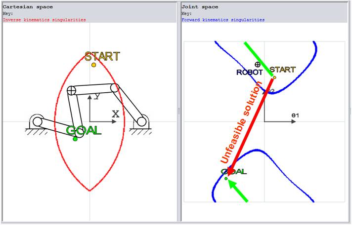
Figure 7. If wraparound is not considered in the path-planning, the algorithm may miss feasible solutions.
In the example shown in figure 7 the path-planner should find a trajectory in the joint space from the starting point to the goal without crossing the forbidden area (in which no solutions for forward kinematics exist). If the planner treats the joint space as a square of side 2π centered at the origin, it will definitively fail when finding a trajectory that links the endpoints, for the start and goal points lie in opposite areas separated by the forbidden points. However, if the planner regards the joint space as a torus - matching the upper limit of the square (corresponding to θ2 = π) to the lower limit of the square (corresponding to θ2 = -π) and matching the right-hand side limit of the square (corresponding to θ1 = π) to the left-hand side limit of the square (corresponding to θ1 = -π) – then it will find a trajectory by wrapping the angle θ2 from π to –π. The path-planning algorithm implemented in the applet takes this issue into account not to miss possible solutions.
After the A* algorithm (regarding the issue mentioned in the previous paragraph) has determined the shortest path – minimum length in joint space, however – between start point and goal, then the applet proceeds to simulate the found trajectory, displaying the robot in the sequence of configurations that will take the end-effector from the initial specified point to the final desired position. A future version of the applet will interpolate the resulting sequence of points to generate a continuous trajectory between the endpoints, choosing the time instants at which the robot should cross each point in order to meet some constraints – not exceeding a maximum angular velocity or torque, for instance. This would be helpful to simulate the inverse dynamics of the robot throughout the whole trajectory and calculate the torques needed to actually perform it, so that this tool could be used in the process of the design of a parallel robot and the choice of the actuators to drive it. Also, methods of path-planning different to the one described here should be implemented in the future.