

Parallel Delta robot
Download the applet
Click here to download the applet of Delta robot simulator.
Instructions of use
The applet for the delta robot has been divided in two areas: on the left-hand side there is a keypad/control window by which the user can choose which kind of analysis is to be performed and control the simulation, on the right hand side there is a graphical window where a scheme of this parallel robot is shown together with three charts that will be used to perform trajectory analyses (see figure 1).
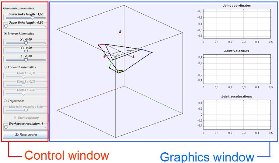
Figure 1. View of the Delta robot simulation.
On
the control window, the geometric parameters of this robot can be changed. The
first sliding bar changes the length of the lower links of the mechanism, which
is set to
It is important to note that although this parallel mechanism has more than one solution for forward kinematics and inverse kinematics problems, the current simulation displays only one solution for both kinematics. The solution that is simulated corresponds to the assembly that most commercial delta robots follow since it has the most interesting mechanical behaviour for industrial tasks. However, the applet will be updated soon to allow the user simulate different assembly modes corresponding to different solutions to its kinematics.
Besides being able to explore the inverse and forward kinematic problems of this robot, the user can also visualize its workspace by modifying the value of the slide bar labelled ‘Workspace resolution’ located at the bottom of the control window. Actually, this action will change the number of points in which an algorithm discretizes the cartesian space to check whether a point belongs to the workspace or not, so a high value of this parameter will provide a fine representation of the workspace while a lower value will result in a coarse approximation. Figure 2 depicts the aspect of the workspace for a resolution value of 20. To hide the workspace, the resolution must be reduced to its lowest value (1).
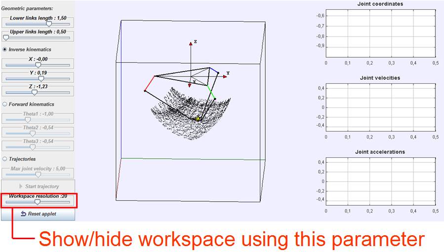
Figure 2. Workspace representation.
The robot can then be moved through its workspace by means of slide bars or directly moving its end-effector with the mouse if inverse kinematic problem is active or, on the other hand, modifying the angular position of the input links dragging them with the mouse or changing the value of the input angles in slide bars if the user prefers to explore the forward kinematic problem (see figure 3). The upper and lower links of the robot may also be modified to see its effect on the volume and shape of the resulting workspace, which is useful in design problems when one wants to know if a specified configuration (in terms of links’ length) allows the robot to reach the points that define a task. The camera angle will change if the user drags the main box where the scheme of the robot is shown, which is good to visualize better the shape of the workspace of the mechanism.
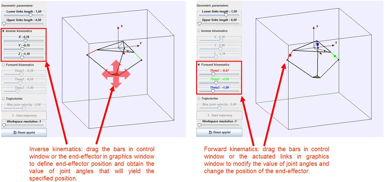
Figura 3. Simulation of inverse (left) and forward (right) kinematics.
In order to see the robot following trajectories in the workspace, the ‘trajectories’ tick must be active. Once activated, the user will not be able to modify the links’ length neither manipulate forward and inverse kinematics menus until ‘trajectories’ tick is disabled again. To perform a trajectory the user must place inside the workspace the desired starting and goal points of the wanted trajectory, and then a maximum joint velocity (in rad/sec) must be chosen by modifying the position of the corresponding sliding bar to limit the angular velocity of the actuated joints to perform the desired trajectory. When properly configured, the trajectory will start after pressing ‘Start trajectory’ button (if at least one of the endpoints lies outside of the workspace the applet will not launch the trajectory and it will display a warning message when pressing this button). The algorithm solves the inverse kinematic problem for both ending and starting points and then connects the resulting angles for initial and final poses (in joint space) by a 4-3-4 trajectory, being limited the maximum angular velocities of the input joints to the value imposed by the user. Since singularities are not taken into account in this path-planning process, the mechanism may behave incorrectly if the planned trajectory crosses any singular configuration. A better algorithm which avoids singularities will be implemented in future versions of the applet, however using a path-planning algorithm which does not provide singularity-free trajectories has the purpose of teaching students the problems of crossing singularities in the trajectory of a parallel robot. Angular position, velocity and acceleration of the three joints are plotted versus time in three different charts on the right side of the main window, where the user can see the designed kinematic profiles (see figure 4).
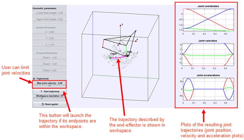
Figure 4. Simulation of a trajectory in the workspace of the parallel manipulator.